Inside the CNN: How Images Become Predictions
Visualize the complete journey of a plant leaf image through each layer of a Convolutional Neural Network
CNN Processing PipelineInteractive
CNN Processing Pipeline
Input Image
224×224×3
Convolution
224×224×32
32 filters (3×3)
Max Pooling
112×112×32
2×2 pool size
Convolution
112×112×64
64 filters (3×3)
Max Pooling
56×56×64
2×2 pool size
Convolution
56×56×128
128 filters (3×3)
Max Pooling
28×28×128
2×2 pool size
Flatten
100,352
Dense + Dropout
512
512 neurons, 0.5 dropout
Output
38
Understanding the CNN Processing Pipeline
The visualization above demonstrates how a CNN processes a plant leaf image through multiple layers to detect diseases. Each step transforms the image in specific ways:
- Input Image: The raw 224×224×3 RGB image is fed into the network with pixel values between 0-255.
- Convolutional Layers: Apply filters to extract features at increasing levels of abstraction - from simple edges to complex disease patterns.
- Pooling Layers: Reduce spatial dimensions while preserving important features, making the model more computationally efficient.
- Flatten Layer: Converts the 3D feature maps into a 1D vector for the fully connected layers.
- Dense Layers: Combine extracted features to make the final disease classification.
- Output Layer: Produces probabilities for each disease class using softmax activation.
Interactive Layer ExplorerAnimated
Convolutional Layer Animation
Convolution Operation
# Convolution operation in Python
import numpy as np

def convolve2d(image, kernel):
    # Get dimensions
    i_height, i_width = image.shape
    k_height, k_width = kernel.shape

    # Output dimensions
    o_height = i_height - k_height + 1
    o_width = i_width - k_width + 1

    # Initialize output
    output = np.zeros((o_height, o_width))

    # Perform convolution
    for y in range(o_height):
        for x in range(o_width):
            # Extract region of interest
            roi = image[y:y+k_height, x:x+k_width]
            # Element-wise multiplication and sum
            output[y, x] = np.sum(roi * kernel)

    return output

# Example: Edge detection kernel
kernel = np.array([[-1, -1, -1],
                   [-1,  8, -1],
                   [-1, -1, -1]])

# Apply to image
feature_map = convolve2d(leaf_image, kernel)
How Convolution Works
Convolutional layers are the core building blocks of CNNs. They apply a set of learnable filters (kernels) to the input image to extract features like edges, textures, and patterns that are characteristic of plant diseases.
Step-by-Step Process
- 1.A small filter (kernel) slides across the input image pixel by pixel
- 2.At each position, element-wise multiplication between the kernel and the covered image patch occurs
- 3.The products are summed to produce a single value in the output feature map
- 4.Multiple filters create multiple feature maps, each detecting different patterns
- 5.ReLU activation introduces non-linearity by replacing negative values with zeros
Mathematical Foundation
The convolution operation is the mathematical foundation of CNNs. For a 2D image input I and a kernel K, the convolution is defined as:
(I * K)(i, j) = ΣΣ I(i+m, j+n) · K(m, n)
This operation slides the kernel K over the input image I, performing element-wise multiplication and summation at each position. The result is a feature map that highlights specific patterns in the image.
Activation functions introduce non-linearity into the network, allowing it to learn complex patterns. The most common activation functions in CNNs are:
ReLU (Rectified Linear Unit)
f(x) = max(0, x)
ReLU replaces all negative values with zero, allowing for faster training and helping prevent the vanishing gradient problem.
Softmax (Output Layer)
Softmax(zi) = ezi / Σ ezj
Softmax converts raw output scores to probabilities that sum to 1, making it ideal for multi-class classification of plant diseases.
Key Takeaways
Feature Extraction
Convolutional layers extract hierarchical features from simple edges to complex disease patterns, with each layer building upon the previous one.
Dimensionality Reduction
Pooling layers reduce spatial dimensions while preserving important disease features, making the model more computationally efficient.
Classification
Fully connected layers combine extracted features to make accurate disease predictions with confidence scores, transforming visual patterns into diagnoses.
Real-world Impact
CNN models can detect plant diseases with 97%+ accuracy up to 10 days earlier than human experts, helping farmers reduce crop losses significantly.
CNN Processing of Plant Leaf ImageInteractive
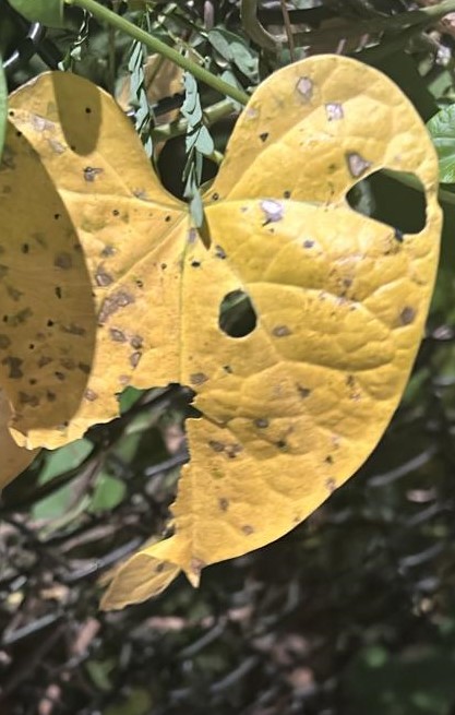
Original Leaf Image
CNN Processing
Analysis of the Leaf Image
The leaf image shows clear signs of disease with multiple small spots and discoloration. Here's how the CNN processes this image:
- Input Processing: The 224×224×3 RGB image is fed into the network. The leaf color, texture patterns, and dark spots are all represented as pixel values between 0-255.
- Feature Extraction (Convolutional Layers): The first convolutional layer with 32 filters detects basic features like the leaf edges, the boundaries of the spots, and the discolored areas. Deeper convolutional layers (64 and 128 filters) identify more complex patterns specific to leaf spot disease.
- Feature Reduction (Pooling Layers): Max pooling layers reduce the spatial dimensions while preserving the important disease features - in this case, the distinctive pattern of spots and discoloration on the leaf.
- Classification: After flattening and passing through dense layers, the model identifies this pattern as characteristic of Leaf Spot Disease with high confidence, based on the specific arrangement, size, and color of the spots on the leaf.